Hado van Hasselt, Arthur Guez, Matteo Hessel, Volodymyr Mnih, David Silver. “Learning values across many orders of magnitude.” In Advances in Neural Information Processing Systems, pp. 4287-4295. 2016. [pdf]
符号系统
| 符号 | 含义 | 符号 | 含义 |
|---|---|---|---|
| $Y_t$ | 目标 (target) | ${\bf W}$ | 标准化层权重 |
| $\tilde{Y}_t$ | 标准化后的目标 | ${\boldsymbol b}$ | 标准化层bias |
| ${\boldsymbol \Sigma}_t$, ${\boldsymbol \mu}_t$ | 学习到的scale和shift | $h_{\boldsymbol \theta}$ | 模型参数 |
| $g(\cdot)$ | 标准化函数 | $f(\cdot)$ | 原函数 |
第二章 Adaptive normalization with Pop-Art
We propose to normalize the targets $Y_t$, where the normalization is learned separately from the approximating function. We consider an affine transformation of the targets
本文的核心思路是将学习标准化与函数拟合两个过程分离开, 具体分离的方式是在原有的函数拟合网络下接一层affine transformation(线性变换)。原有的函数负责学习函数拟合, 而下接的一层线性变换层负责”跟踪”|学习标准化的参数。
We can then define a loss on a normalized function $g(X_t)$ and the normalized target $\tilde{Y}_ T$. THe unnormalized approximation for any input $x$ is then given by $f(x) = {\boldsymbol \Sigma} g(x) + {\boldsymbol \mu}$, where $g$ is the normalized function and $f$ is the unnormalized function.
Thereby, we decompose the problem of learning an appropriate normalization from learning the specific shape of the function. The two properties that we want to simultaneosly achieve are
(ART) to update scale ${\boldsymbol \Sigma}$ and shift ${\boldsymbol \mu}$ such that ${\boldsymbol \Sigma}^{-1} (Y - {\boldsymbol \mu})$ is approproately normalized, and
(POP) to preserve the outputs of the unnormalized function when we change the scale and shift.
其中ART负责学习标准化参数, 而POP负责保障任何的标准化参数下总能从标准化后的结果复原原始的输出。有了两点的结合就能实现针对任意输出情况下用合适的标准化参数进行normalization, 与此同时保障不破坏已经学习到函数拟合结果。
2.1 POP: Preserving outputs precisely
Unless care is taken, repeated updates to the normalization might make learning harder rather than easier because the normalized targets become non-stationary. More importantly, whenever we adapt the normalization based on a certain target, this would simultaneously change the output of the unnormalized function of all inputs.
本段解释了提出POP的motivation。可想而知, 如果无法保障原始(未标准化)的target不能被复原的话, 那么一旦在学习时采用了不同的标准化参数, 原有学习到的模型将受到影响(破坏)。举例而言, 假设首先学习到的模型是通过原始target范围在$[0, 1]$内, 而后出现的样本target范围在$[10, 100]$, 将其标准化至$[0, 1]$内后作为新的样本训练已有模型, 那么原来模型的所给出的$[0, 1]$范围结果将受到”波及”。
The only way to avoid changing all outputs of the unnormalized function whenever we update the scale and shift is by changing the normalized function $g$ itself simultaneously. The goal is the preserve the outputs from before the change of normalization, for all inputs. This prevents the normalization from affecting the approximation, which is appropriate because its objective is solely to make learning easier, and to leave solving the approximation itself to the optimization algorithm.
解决此问题的唯一办法就是在更新标准化参数的同时更新原有标准化前的输出。标准化的目的在于使得训练集在差不多的规模内从而使模型训练更为容易, 需要防止标准化影响模型训练本身。
Without loss of generality the unnormalized function can be written as
其中$g_ { {\boldsymbol \theta}, {\bf W}, {\boldsymbol b} } (x) = {\bf W} h_ { {\boldsymbol \theta} } (x) + {\boldsymbol b}$ 为标准化函数, 而$h_ { {\boldsymbol \theta} } (x)$ 是函数拟合的网络(non-linear)。
It is not uncommon for deep neural networks to end in a linear layer, and the $h_ { {\boldsymbol \theta} }$ can be the output of the last (hidden) layer of non-linearities. Alternatively, we can always add a square linear layer to any non-linear function $h_ { {\boldsymbol \theta} }$ to ensure this constraint, for instance initialized as ${\bf W}_ 0 = {\bf I}$ and ${\boldsymbol b}_ 0 = {\boldsymbol 0}$.
本段解释了网络架构, 一般而言DNN的最后一层(输出层)均具备线性激活, 即满足以上的条件; 若不然, 则可以在原有网络的基础上加上一个线性层(本层参数规模为$k\times k | k$, $k$为输出的层的神经元数量), 不改变网络架构的同时满足了以上的条件。
Proposition 1. Consider a function $f: \mathbb{R}^n \rightarrow \mathbb{R}^k$ as
where $h_ {\boldsymbol \theta}: \mathbb{R}^n \rightarrow \mathbb{R}^m$ is any non-linear function of $x\in \mathbb{R}^n$, ${\boldsymbol \Sigma}$ is a $k\times k$ matrix, ${\boldsymbol \mu}$ and ${\boldsymbol b}$ are $k$-element vectors, and ${\bf W}$ is a $k\times m$ matrix. Consider any change of the scale and shift parameters from ${\boldsymbol \Sigma}$ to ${\boldsymbol \Sigma}_ \text{new}$ and from ${\boldsymbol \mu}$ to ${\boldsymbol \mu}_ \text{new}$, where ${\boldsymbol \Sigma}_ \text{new}$ is non-singular. If we then additionally change the parameters ${\bf W}$ and ${\boldsymbol b}$ to ${\bf W}_ \text{new}$ and ${\boldsymbol b}_ \text{new}$, defined by
then the outputs of the unnormalized function $f$ are preserved precisely in the sense that
以上的Proposition表明只要采用适当的标准化参数变换方案总能保证原函数拟合的结果保持不变。其中适当的变化方案即以上给出的${\bf W}_ \text{new}$与${\boldsymbol b}_ \text{new}$的更新方案。
For the special case of scalar scale and shift, with ${\boldsymbol \Sigma} \equiv \sigma {\bf I}$ and ${\boldsymbol \mu} \equiv \mu {\boldsymbol 1}$, the updates to ${\bf W}$ and ${\boldsymbol b}$ become ${\bf W}_ \text{new} = (\sigma/\sigma_\text{new}) {\bf W}$ and ${\boldsymbol b}_ \text{new} = (\sigma {\boldsymbol b} + {\boldsymbol \mu} - {\boldsymbol \mu}_ \text{new})/\sigma_ \text{new}$. After updating the scale and shift we can update the output of the normalized function $g_ { {\boldsymbol \theta}, {\bf W}, {\boldsymbol b} } (X_ t)$ toward the normalized $\tilde{Y}_ t$, using any learning algorithm.
以上给出了特例, 即当scale和shift均为标量。按以上规则更新了标准化参数后, 根据Proposition 1可知原来的输出在新的标准化参数下并不会改变, 而新的训练数据通过新的标准化参数处理后即可用于对函数拟合模型(即$h_ { {\boldsymbol \theta} }$)的训练。
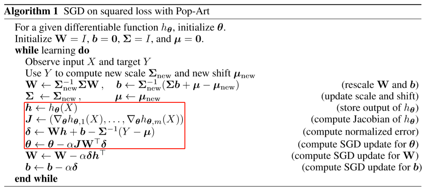
Algorithm 1 is an example implementation of SGD with Pop-Art for a squared loss. It can be generalized easily to any other loss by changin the definition of ${\boldsymbol \delta}$. Notice that ${\bf W}$ and ${\boldsymbol b}$ are updated twice: first to adapt to the new scale and shift to preserve the outputs of the function, and then by SGD. The order of these updates is important because it allows us to use the new normalization immediately in the subsequent SGD update.
在此基础上, 算法1以MSE为loss函数, SGD为optimizer为例阐述了如何实现Pop-Art算法。其中主要分为三个阶段:
- 更新标准化参数(Pop)
- 更新函数拟合模型内层($h_ { {\boldsymbol \theta} }$), (算法中红框标注部分)
- 由SDG更新标准化层参数
小结: 本节主要阐述了Pop-Art算法中的Pop部分, 即如何更新标准化参数以保证后续的训练可以保障不影响已有输出的结果。另一方面, 通过算法1给出了结合Pop-Art的网络更新流程, 其中标准化层的参数将被更新两次, 第一次为保障Pop, 第二次为优化算法下的参数更新。
2.2 ART: Adaptively rescaling targets
前一节中介绍了标准化参数更新过程中保障已有输出不变的基本思路, 而本节将具体给出如何进行标准化, 即Art: Adaptively rescaling targets的内涵。
A natual choice is to normalize the targets to approximately have zero mean and unit variance. For clarity and conciseness, we consider scalar normalizations. If we have data $\{ ( X_ i, Y_ i ) \}_ {i=1}^t$ up to some time $t$, we then may desire
This can be generalized to incremental updates
Here $\nu_t$ estimates the second moment of the targets and $\beta_t\in [0, 1]$ is a step size. If $\nu_t -\mu_t^2$ is positive initially then it will always remain so, although to avoid issues with numerical precision it can be useful to enforce a lower bound explicitly by requiring $\nu_t -\mu_t^2 \geq \epsilon$ with $\epsilon >0$. For full equivalence to above one we can use $\beta_t = 1/t$. If $\beta_t = \beta$ is constant we get exponential moving averages, placing more weight on recent data points which is appropriate in non-stationary settings.
自然地, 标准化的思路是将现有的数据统一到均值为0, 方差为1的规模, 考虑到数据本身是源源不断出现的, 更一般地可以用以上的增量式更新方式update均值($\mu_t$)和标准差($\sigma_t$)。两种特殊情况: 1) $\beta_t = 1/t$, 则每个样本的权重一致; 2) $\beta_t=\beta$为定值, 则意味着指数式的滑动平均, 最近的样本具有更高的权重, 适用于non-stationary的情况。另一方面, 从数值精度考虑, 有必要为更新的$\sigma_t^2$(即$\nu_t - \mu_t^2$)设置一个下限, $\epsilon$, 以防出现除0的情况。
A constant $\beta$ has the additional benefit of never becoming negligibly small. Consider the first time a target is observed that is much larger than all previously observed targets. If $\beta_t$ is small, our statistics would adapt only slightly, and the resulting update may be large enough to harm the learning. If $\beta_t$ is not too small, the normalization can adapt to the large target before updating, potentially making learning more robust.
本段进一步解释了$\beta$取定值的一个优点。假设$\beta$逐步递减至较小值时, 若此时首次出现一个相对大的目标值, 由于$\beta$太小, 导致新纳入的样本对已有的统计量($\mu$和$\sigma$)的影响很微小, 可以近似认为统计量不变, 那么根据算法1, 其中关键步骤1对统计量的更新就可以忽略, 此时第二步中由于新的样本target值过大导致对模型的训练产生大的影响。相反, 如果$\beta$不太小, 这样的情况下, 在函数拟合网络($h_ { {\boldsymbol \theta} }$)之前, 较大的target值将由统计量的更新而削弱进而增强模型整体的鲁棒性。
Proposition 2. When using updates above to adapt the normalization parameters $\sigma$ and $\mu$, the normalized targets are bounded for all $t$ by
For instance, if $\beta_t = \beta = 10^{-4}$ for all $t$, then the normalized target is guaranteed to be in $(-100, 100)$.
以上的Proposition表明了上述增量式统计参数更新下获得的target范围与$\beta_t$的关系, 对于参数选择具有一定指导效果。
It is an open question whether it is uniformly best to normalize by mean and variance. In the appendix we discuss other normalization updates, based on percentiles and mini-batches, and derive correspondences between all of these.
以上给出的是均值|标准差的标准化方式, 该种方式是否具有普适性仍然是一个开放式的问题。作者在附录中讨论了其他的标准化方式, 尤其是mini-batches值得关注。
小结: 本节介绍了Pop-Art中的”Art”部分, 即自适应target缩放。提出了一个增量式的标准化方式, 其中通过参数$\beta_t$的不同取值方式可以应对不同的场景。针对target non-stationary的情形, 建议使用$\beta_t$为定值, 以增强模型鲁棒性, 便于应对target出现突然的变化。(否则, 若$\beta_t$随$t$减小, “异常”的target对统计参数的影响将很小, 但对模型更新的”伤害”却很大。)
2.3 An equivalence for stochastic gradient descent
We now step back and analyze the effect of the magnitude of the errors on the gradients when using regular SDG. This analysis suggests a different normalization algorithm, which has an interesting correspondence to Pop-Art SGD.
在本节中, 作者将讨论跨度广泛的target对SGD算法的影响, 并提出相应的标准化算法。该算法与前述的Pop-Art SGD (算法1)有着有趣的关联。
We consider SGD updates for an unnormalized multi-layer function of form $f_ { {\boldsymbol \theta}, {\bf W}, {\boldsymbol b} } (X) = {\bf W} h_ { \boldsymbol \theta}(X) + {\boldsymbol b}$. The update for the weight matrix ${\bf W}$ is
where ${\boldsymbol \delta}_ t = f_ { {\boldsymbol \theta}, {\bf W}, {\boldsymbol b} } (X) - Y_t$ is gradient of the squared loss, which we here call unnormalized error. The magnitude of this update depends linearly on the magnitude of the error, which is appropriate when the inputs are normalized, because then the ideal scale of the weights depends linearly on the magnitude of the targets.
本段着手分析最后一层的权重(${\bf W}$)的更新与误差项($f_ { {\boldsymbol \theta}, {\bf W}, {\boldsymbol b} } (X) - Y_t$)之间的关系, 指出权重的更新规模与误差项的规模呈线性关系。进一步误差项本身的规模又与target的规模呈线性关系。正常情况下(即target的规模在相对小的范围内时), 以上的更新是没问题的。
Now consider the SGD update to the parameters of $h_ { {\boldsymbol \theta} }$, ${\boldsymbol \theta}_ t = {\boldsymbol \theta}_ {t-1} - \alpha {\boldsymbol J}_ t {\bf W}_ {t-1}^\intercal {\boldsymbol \delta}_ t$ where ${\boldsymbol J}_ t = ( \nabla h_ { {\boldsymbol \theta}, 1 } (X), \ldots, \nabla h_ { {\boldsymbol \theta}, m } (X) )^\intercal$ is the Jacobian for $h_ { {\boldsymbol \theta} }$. The magnitudes of both the weights ${\bf W}$ and the erros ${\boldsymbol \delta}$ depend linearly on the magnitude of the targets. This means that the magnitude of the update for ${\boldsymbol \theta}$ depends quaratically on the magnitude of the targets. There is no compelling reason for these updates to depend at all on these magnitudes because the weights in the top layer already ensure appropriate scaling. In other words, for each doubling of the magnitudes of the targets, the updates to the lower layers quadruple for no clear reason.
进一步, lower layer的网络参数(${\boldsymbol \theta}$)更新幅度根据公式既与${\bf W}$规模呈线性关系, 又与误差项规模呈线性关系, 两者均与target的规模呈线性关系并且是相乘的关系, 综合导致lower layer网络参数更新幅度与target的规模呈平方关系。而事实上并没有显著的理由保证如此的关系。(相反这可能造成对参数的”破坏”)
注: 一般多层网络中, lower layer | upper layer的概念是根据搭建的顺序而言, 接近Input的为lower layer, 而接近Output的为upper layer。(此前对这两者理解正好相反🤣)
This analysis suggests an algorithmic solution, which seems to be novel in and of itself, in which we track the magnitude of the targets in a separate parameter $\sigma_t$, and then multiply the updates for all lower layers with a factor $\sigma_t^{-2}$. A more general version of this for matrix scallings is given in Algorithm 2.
根据以上的分析, 作者提出了相应的解决方案, 即跟踪target的规模$\sigma_t$, 并对lower layer的更新相应乘以$\sigma_t^{-2}$从而消除此处引入的target规模的影响。具体的算法流程在Algorithm 2中给出(其中${\bf W} \leftarrow {\bf W} - \alpha {\boldsymbol \delta} {\boldsymbol g}^\intercal$中${\boldsymbol g}$应该是${\boldsymbol h}$)。
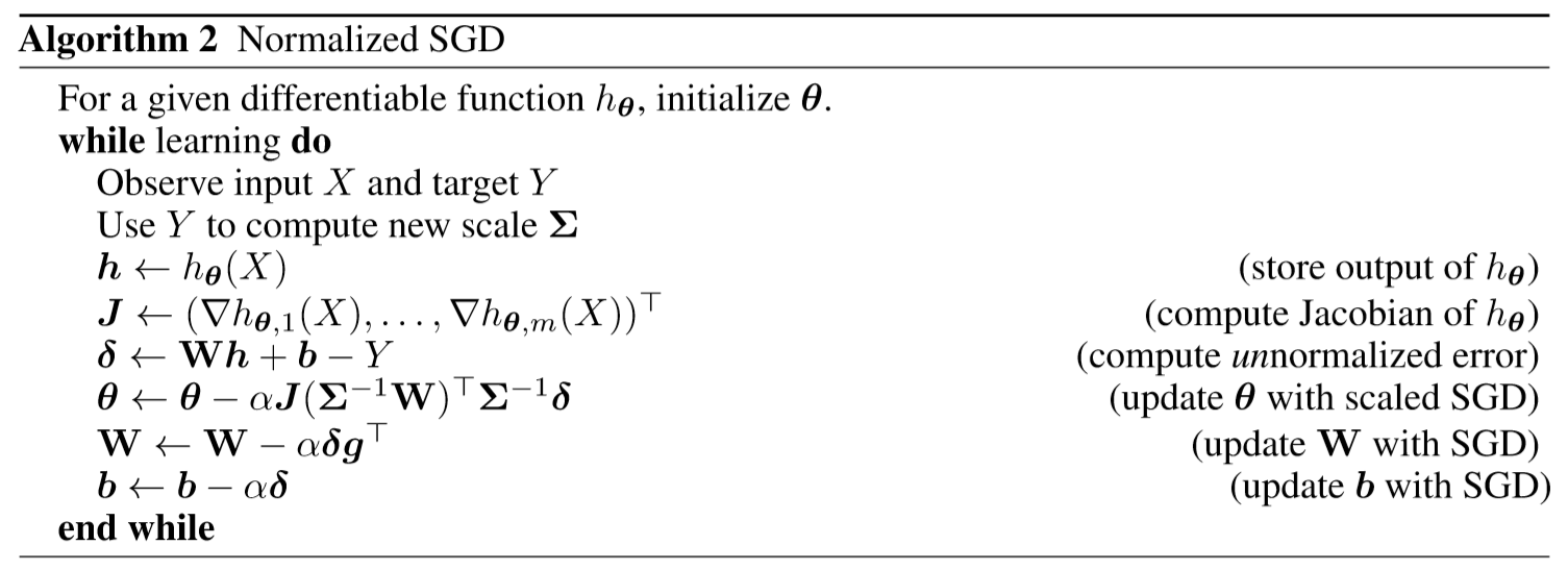
算法2中的核心步骤是${\boldsymbol \theta} \leftarrow {\boldsymbol \theta} - \alpha {\boldsymbol J} ( {\color{red} {\boldsymbol \Sigma} ^{-1} } {\bf W})^\intercal {\color{red} {\boldsymbol \Sigma}^{-1} } {\boldsymbol \delta}$, 其中对${\bf W}$和${\boldsymbol \delta}$分别做了”半标准化”处理, 即将其magnitude置为一。
小结: 至此, 作者提出了第二个算法。该算法的思路不同于算法1对target进行标准化, 而是看准target规模对模型参数update的影响会分别通过误差项(${\boldsymbol \delta}_ t$)和top layer权重(${\bf W}$)引入而造成quadratic的影响, 考虑在lower layer模型参数update中消除该影响。
We prove an interesting, and perhaps surprising, connection to the Pop-Art algorithm.
Proposition 3. Consider two functions defined by
where $h_ { {\boldsymbol \theta} }$ is the same differentiable function in both cases, and the functions are initialized identically, using ${\boldsymbol \Sigma}_ 0 = {\bf I}$ and ${\boldsymbol \mu}={\bf 0}$, and the same initial ${\boldsymbol \theta}_ 0$, ${\bf W}_ 0$ and ${\boldsymbol b}_ 0$. Consider updating the first function using Algorithm 1 (Pop-Art SGD) and the second using Algorithm 2 (Normalized SDG). Then, for any sequence of non-singular scales $\{ {\boldsymbol \Sigma}_ t \}_ {t=1}^\infty$ and shift $\{ {\boldsymbol \mu}_ t \}_ {t=1}^\infty$, the algorithms are equivalent in the sense that 1) the sequences $\{ {\boldsymbol \theta}_ t \}_ {t=0}^\infty$ are identical, 2) the outputs of the functions are identical, for any input.
以上的Proposition阐述了算法2和算法1的等效性。当初始的上下层权重一致时, 并且算法1中初始的统计算法按照”单位化”设置, 则两个算法下在任意时刻的结果均是一致的。
The proposition shows a duality between normalizing the targets, as in Algorithm 1, and changing the updates, as in Algorithm 2. This allows us to gain more intuition about the algorithm. In particular, in Algorithm 2 the updates in top layer are not normalized, thereby allowing the last linear layer to adapt to the scale of the targets. That said, these methods are complementary, and it is straightforward to combing Pop-Art with other optimization algorithms than SGD.
再次强调以上Proposition的重要性, 保障了两个算法间的对偶性。另一方面, 算法2中的top layer并未进行标准化处理, 从而保留了其适应target的调整空间。Proposition表明Pop-Art算法本身可以作为对其他优化算法的一个补充。
小结: 本节提出了重要的Proposition, 阐述了算法2和算法1的等效性, 因此Pop-Art算法可以作为对其他优化算法的一个补充。
总结与思考
本文考虑强化学习中target跨度大而导致模型学习效果差的问题进行了研究, 提出了Pop-Art算法解决该问题。其算法的核心包括两个部分: 1) Pop (Presering outputs precisely): 即无论标准化参数如何变化, 已有的输出不会变化; 2) Art (Adaptive rescaling target): 即自适应目标值放缩, 保障新的目标值能合理的放缩标准化。此外, 本文还分析了target跨度大导致模型学习效果差的原因: target的跨度影响将”平方式”地影响lower layer的参数更新。在此基础上, 作者提出了针对lower layer更新的修正算法, 并证明了该算法与前述Pop-Art算法的等效性。
疑问: 强化学习算法中多为mini-batch的训练模式, 那么在随机选取的batch中可能出现如下的情况: $[ a_1, \ldots, a_n, b_1, \ldots, b_m]$。其中$a$, $b$序列分别在不同的范围, 同组中彼此差异仅体现在小数点后3位, 而两组间的差异为个位数。在这种情况下, 标准化处理是否能够有效区分组内的差异呢?此batch的处理是否应该将样本逐一输入进行处理?
此疑问在文章的附加部分中有所涉及, 即需要替换”Art”部分。